Weitere Optionen
Ulli (Diskussion | Beiträge) Keine Bearbeitungszusammenfassung |
Ulli (Diskussion | Beiträge) Keine Bearbeitungszusammenfassung |
||
| Zeile 18: | Zeile 18: | ||
At l=40° e.g. we have some approaching clouds at low level, that are not resolved by my small antenna ,two escaping with high intensity and one nearly at rest relative to the earth. | At l=40° e.g. we have some approaching clouds at low level, that are not resolved by my small antenna ,two escaping with high intensity and one nearly at rest relative to the earth. | ||
Taking such records every 5° of galactic longitude and arranging the data by a specialized program, I obtain diagrams like fig.2: it is a contourplot, that shows in the z-axis colour encoded (here unfortunately only grey steps) the intensity over the velocity of the HI-clouds for the galactic plane, that can be seen from my station. The x-axis is calibrated in km/s, corresponding to the velocity of approach (-) or recession (+) of the observed hydrogen cloud following the formula | Taking such records every 5° of galactic longitude and arranging the data by a specialized program, I obtain diagrams like fig.2: it is a contourplot, that shows in the z-axis colour encoded (here unfortunately only grey steps) the intensity over the velocity of the HI-clouds for the galactic plane, that can be seen from my station. The x-axis is calibrated in km/s, corresponding to the velocity of approach (-) or recession (+) of the observed hydrogen cloud following the formula | ||
v = c<math>\triangle\nu/nu</math> see /3/ Kraus, page 8-88. | v = c<math>\triangle\nu/\nu</math> see /3/ Kraus, page 8-88. | ||
<math>\nu</math>: rest frequency, <math>\nu</math>=1420.406 MHz | <math>\nu</math>: rest frequency, <math>\nu</math>=1420.406 MHz | ||
Version vom 8. Oktober 2009, 15:48 Uhr

Observation of Neutral Hydrogen (HI) with a small parabolic dish Part I: Observations Ernst Lankeit, Oktober 2006 elankeit@t-online.de
In /1/ I gave a description of my 2.20m parabolic antenna and in /2/ were observations of the sun at 1420 Mhz. Here I will describe the results of HI-observation and in Part II I give some technical hints to the receiving equipment.
1 The difficult approach to success For the first tests the receiving chain consisted of a LNA and a homebrew converter followed by my 137 MHz receiver at fixed frequency and 1MHz bandwidth used for sun observation. What did I see or measure? Nothing! When moaning about this failure, our member H. OSER showed to me his pretty records of HI-lines, taken by his 3m dish. He was convinced of getting the same results with my smaller antenna and reproved: „May be, you are searching at wrong place with wrong frequency and wrong bandwidth!“. So I
- added galactic coordinates to my controlling SW see /1/,
- rebuilt my receiver to sweep 1419 MHz to 1422 MHz under control of a PC and
- added a switchable IF-bandwidth of 15 KHz and 30 KHz. (that are 3 lines, but they took 1 year, details see below).
After that trouble I am now able to record strong HI-profiles – thanks to Mr. OSER!
2 Results: HI-profiles of the galactic plane Fig.1 shows a row of records, taken at the particular galactic longitude at galactic latitude b=0. The ordinate is calibrated in volt, because an absolute calibration of my station is missing until now, but a coarse estimation gives 1V~20K of emission brightness temperature. The x-axis is the deviatiation from the HI-restfrequency in MHz, rest frequency =1420.406 MHz. The IF-bandwidth is 30 KHz, integration time of the DC-amp is 2s. Frequency distance of reading is 20 KHz, so one scan takes 71 measurements, done by the PC. At l=40° e.g. we have some approaching clouds at low level, that are not resolved by my small antenna ,two escaping with high intensity and one nearly at rest relative to the earth. Taking such records every 5° of galactic longitude and arranging the data by a specialized program, I obtain diagrams like fig.2: it is a contourplot, that shows in the z-axis colour encoded (here unfortunately only grey steps) the intensity over the velocity of the HI-clouds for the galactic plane, that can be seen from my station. The x-axis is calibrated in km/s, corresponding to the velocity of approach (-) or recession (+) of the observed hydrogen cloud following the formula
v = c see /3/ Kraus, page 8-88.
: rest frequency, =1420.406 MHz So v=100 km/s corresponds to ~470 KHz.Such a survey needs some days of observation (sometimes I have to work a little bit to feed my family!), but the error originating in the changing position of the earth is neclectable in fig.2. These diagrams you can find e.g. in /4/ Verschuur, Kellermann, naturally in an much higher resolution. That contourplot is not a picture of our galaxy, but shows regions of the milky way with coherent velocities.
3 Estimate of the position of the HI-clouds Most interesting is now the answer to the question: where are these hydrogen clouds and how far can I see with my tiny parabola? To solve this problem I had to warm up old knowledge of geometry, help I found in /3/ Krauss and more detailed in /5/Carroll. The basic idea behind the following calculation goes back to van de Hulst, Muller and Oort in the middle of the last century: From different measurements we know the curve of differential rotation of the milky way galaxy, so tangential velocity at a point as function of the distance of this point to the galactic center. For the points in fig.2 we have the radial velocity relative to the earth or sun. Using the geometry of the system galactic center, sun and HI-cloud it is possible , to calculate the angular velocity of the cloud relative to the galactic center and with the above mentioned differential rotation curve we can estimate the distance of the cloud to the galactic center and at least we can calculate the distance to the sun. Hoping, that other amateur observers will measure HI-profiles I’ll derivate here the formulas I used, so we could compare our results.
The rotation curve of the milky way galaxy: As basic data I used the values of rotation speed in /5/ figure 22.27, my used mean values are sketched in fig.3. From this I derived the angular velocity as function of distance to the galactic center in fig.4 ; in rad/s; R: kpc 1kpc=3.08*10 km. For values R>8 kpc the error bars in fig.3 grow extremely. For the sun the IAU standard values = 8.5 kpc and = 220 km/s are used. A similar curve to fig.4 can be found e.g. in /3/ fig. 8-63.
Angular velocity of the HI-cloud: In fig.5 means: C the galactic center, S the Sun, H the investigated hydrogen cloud, l is the galactic longitude (earlier l ), and show the direction of the rotation of the sun about the galactic center. From fig.5 we find the relative radial velocity of H:
= cos - sinl
where sinl is the angular velocity of the sun. Defining the angular velocity as we get
= r cos - sinl /1
For calculating the distance x we find two triangles:
x = sinl and x =r cos leading to relation sinl = r cos. Substituting this into /1 we have
= sinl - sinl
= (-) sinl
and at least
= /(sinl)+ /2
Calculating /2 for a desired point in fig.2 in units rad/s we can find in fig.4 the adequate distance r of this point to the galactic center.
Distance Sun – HI-cloud: Referring to fig.6 we find the relations
a=cosl, b=sinl, , y= /3
d = a-y, substituting /3 we get after all the desired distance
d = cosl– /4
This procedure I applied to the regions 1 to 5 in fig.2, every 10 deg of longitude l. The so calculated distances S – H plotted for 20 to 220 deg give the fig.7 with the results:
- the regions in fig.2 describe apparently different arms of the milky way galaxy region 3 represents the radiation of two arms 3a and 3b region 1 may be the “Outer arm”, region 3a the local arm of our sun, called “Orion arm”, region 3b the “Perseus arm” and the week region 2 traces of the “Zwischenarm” (??) for d>8kpc the error in fig.4 is high, so the measured distance of arm 1 is questionable. So – if I did not make a severe failure – it is really possible, to get an impression of a part of our milky way in kpc-distances using a 2m-dish and amateur gear! For me this is still an exiting experience! The only explanation I can find is, that these HI-clouds are so huge, that they fill nearly the whole aperture of my antenna pushing the output to 2..3 dB above noise.
References Part I
/1/ Lankeit, E.: My New Microwave Telescope: Some Hints to Construction and Electronics, ERAC Newsletter 28, September 2005
/2/ Lankeit, E.: Traces of the 2004 Oktober 20 Solar X-Ray Flare, ERAC Newsletter 28, September 2005
/3/ Kraus, J.D.: Radioastronomy 2nd Ed., Cygnus-Quasar Books
/4/ Verschuur, G.L. Kellermann, K.I.: Galactic and Extragalactic Radio Astronomy, Springer 1988
/5/ B.W. Carroll, D.A. Ostlie: An Introduction to Modern Astrophysics, Addison Wesley 1995
Observation of Neutral Hydrogen (HI) with a small parabolic dish
Part II: Equipment Die aufgeführten Zeichnungen sind aus dem NL zu entnehmen, uKu
Ernst Lankeit, Oktober 2006 elankeit@t-online.de
1 Antenna The Antenna fig.1 is a parabolic dish, diameter 2.2m f/D=0.35, details of the mounting see /1/ Part 1. The feed is a simple circular feed horn 160mm diameter and 275mm long, with a ~/4 probe. The first stage of the LNA is mounted direct to the N-port of the feed horn. Via a second /4 probe a noise signal for calibration is injected.
2 Receiver The 21cm receiver consists of three parts: 2 LNA stages at the antenna fig.2 a converter unit from 1420.4 down to 137.9 MHz fig.3 and 4 and the tuneable receiver 137 to 140 MHz.
3 LNA Two LNA are necessary for low noise figure and to compensate the attenuation of 10m H100-coax cable into my lab. The 1. LNA is a 1.3 GHz cavity-LNA see /1/ tuned to 1.4 GHz, the originally FHX35lg meanwhile replaced by a ATF 36077. The noise figure is NF~0.50 dB at 1.42 GHz. The second stage is the older stripline amplifier by DJ9BV /2/ corresponding to the original circuit for 1.3 GHz. NF~0.7 at 1.4 GHz. Meanwhile I have developed some better solutions for the LNA specialised for 21 cm, but the measurements in part 1 were done with this configuration. The data at transmissionlines mean impedance/electrical length.
4 Converter Unit 1420 MHz to 138 MHz Fig.1 and 2 in part I show a velocity range of +/- 150 km/s corresponding to a frequency range of 1.4 MHz. Such a bandwidth is easily achieved by a transverter at fixed frequency, so the tuning can be done in the last stage at ~138 MHz. The converter is home-made and especially designed for 21cm receiving, some suggestions I have taken from /3/. The 1. rf-stage is the result of simulation using ANSOFT DESIGNER, it is etched on 0.79mm-PTFE substrate. The 2. rf and mixer is etched on 1.5mm-FR4 using helical filters. The noise figure of the first stage is NF=0.6 dB, but it is drastically reduced by the high attenuation of the following helical filter F1 to 1.5dB (I optimised the 1. stage to minimum noise, but that is not very clever in this case: it is better, to optimise the input reflection coefficient and to use a resonator with lower attenuation, e.g. a pipe cap filter instead of F1. The overall NF is determined by NF and gain of the 2 LNA!). The mixer is followed by a diplexer at 137 MHz and a U310 for higher IP. The local oscillator power is amplified by an ERA3, the following TOKO 1130 is reduced by 0.5 winding, so the matching to the mixer is not the best, but all works nicely! The overall gain is 36 dB, the 3 dB-bandwidth is 3 MHz. That is more than enough. To avoid overload of the following receiver a 3 dB fixed attenuator is added. The LO chain fig.4 follows the standard circuit, see e.g. /3/. The XO oscillates at 106.875 MHz, followed by a quadrupler to 427.500 MHz and a tripler to the end frequency of 1282.500 MHz. 1420.40 minus 1282.50 gives the receiver frequency of 137.90 MHz.
5 Tuneable Receiver The tunable receiver is a superhet with a single IF of 10.7 MHz, the RF-stages of it equal that swept frequency receiver for sun observation described in /4/ with two main differences: there I needed a high sweeping frequency to maintain 25 measurements on 40 frequencies per second, that was to fast for a cheap phased locked loop (PLL) oscillator. In HI-observation with integration times >1s a computer controlled PLL does the job. And regarding the small tuning band of only ~1.5 MHz I could realise the rf-stages at fixed frequency of 137.9 MHz without tuning. The small IF-bandwidth of 15 KHz and 30 KHz is realised by x-tal filters at 10.7 MHz. Regarding the limited resolution in space of my antenne and following the velocity range of the observed clouds a bandwidth of 30 KHz gives sufficient resolution. Recording in 20 KHz-steps, I need 71 measurements for one sweep. Using an integration time of 1s I take a probe every 2s, so a sweep needs ~140s. With 15 KHz I practically need double the time and dont find smaller ripples in the HI-clouds. Important is an automatic gain control at every frequency step, to compensate ripples in the overall characteristic of antenna, filters and amplifiers. When the antenna looks to a cold point at the sky or into 50 ohms a flat line over the frequency has to be recorded. This gain adjust is done by the PC and a 12 bit-DAC, adjusting the gain of the 2.IF. It should be possible, to use an amateur receiver on the 2m-band, provided that it offers the above IF-bandwidth. The converter stages can easily be tuned to the desired frequencies.
6 Software Although an analog control of the receiver is possible (tuning by a sawtooth generator Mr. OSER e.g. gets excellent HI-profils) I prefer a complete control by the PC. For data recording we need anyhow the computer, so this stupid box can even do the rest. My controlling program I have written in DELPHI 6, using Qinn-Curtis tools for easier implementation of real time routines. It uses a ISA-card with 12 bit ADC and DAC. The program (see screen shot

as example)
- tunes and adjusts the receiver
- gives a real time plot of the received HI-profile
- controls a noise source for calibration
- records the output data
- writes a line plot for printing, see part I Fig.1
- collects the data of repeated observations to create contourplots like part I fig.2
This program runs in multitascing together with the controlling tool of the antenna position. Unfortunately the above realisation of HI-observation is not a beginners project, but if anybody is interested and needs help, send a mail to me. May be the existing layouts or the software can be adapted to your purposes.
References Part II
/1/ Cerveny, Schreyer: Cavity Preamp for 1.3 GHz, DUBUS 1/1997
/2/ Bertelsmeier, R.: HEMT LNAs for 23cm, DUBUS 4/1993
/3/ Kuhne, M.: 1.3 GHz Transverter MKII, DUBUS 2/2000
/4/ Lankeit, E.: Dynamic Solar Spectra, Part 2 Equipment, ERAC Newsletter 23, October 2002